Burst is a feature that allows satisfying queue requirements for additional bandwidth even if the required rate is bigger than MIR (max-limit) for a limited period of time.
Burst can occur only if average-rate of the queue for the last burst-time seconds is smaller than burst-threshold. Burst will stop if average-rate of the queue for the last burst-time seconds is bigger or equal to burst-threshold.
The burst mechanism is simple — if a burst is allowed max-limit value is replaced byburst-limit value. When the burst is disallowed max-limit value remains unchanged.
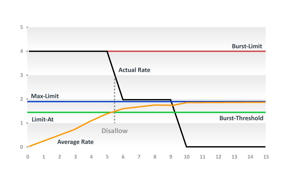
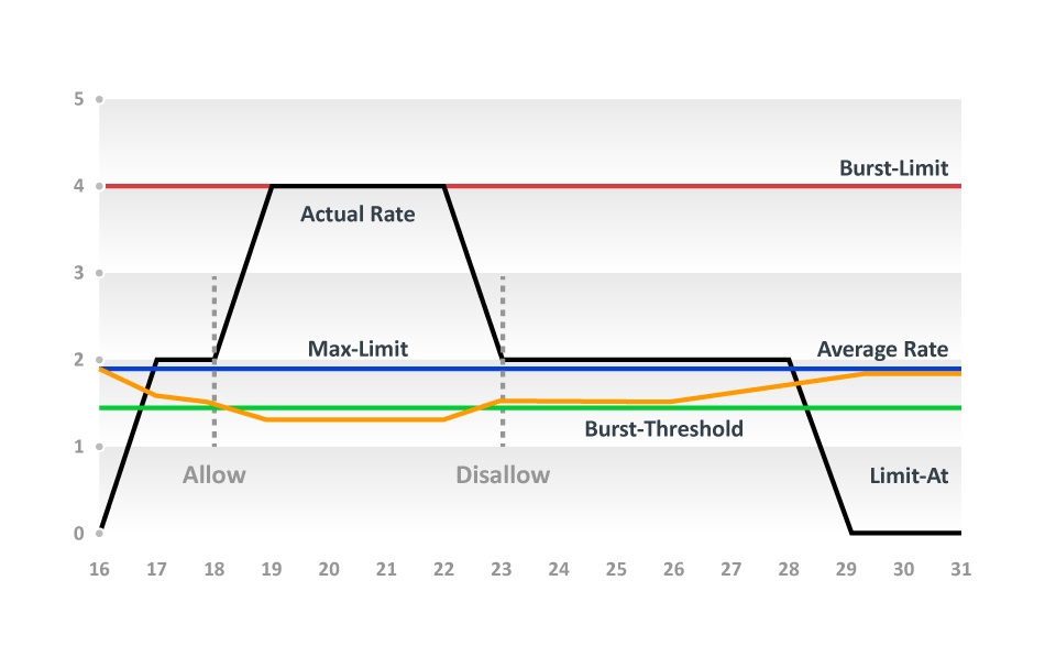
The average rate is calculated every 1/16 of burst time so in this case 1s
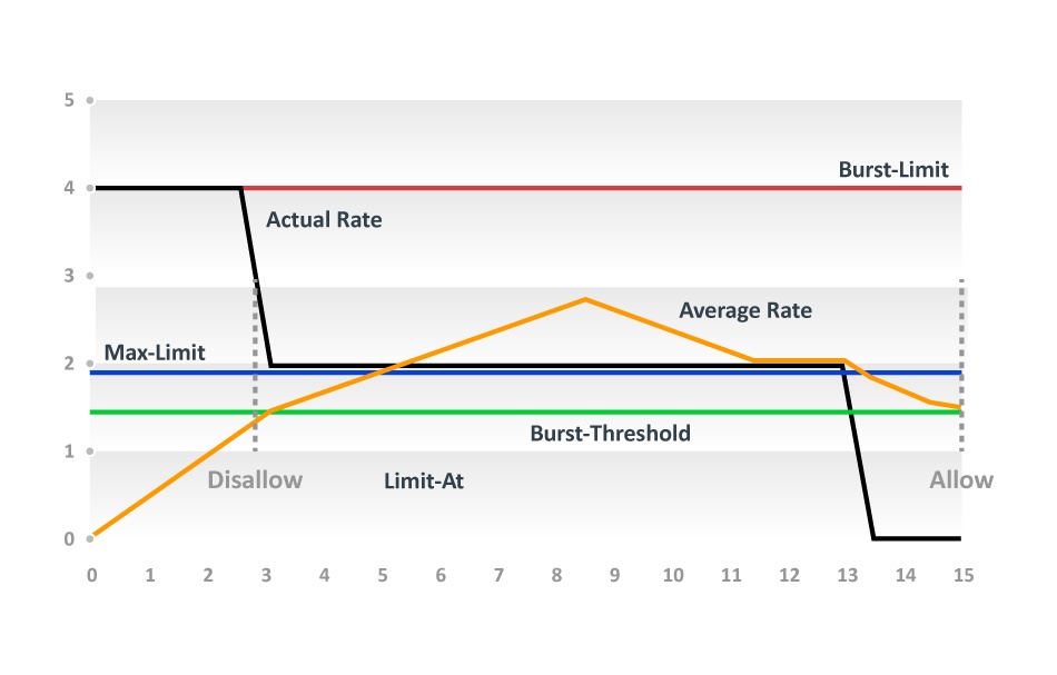
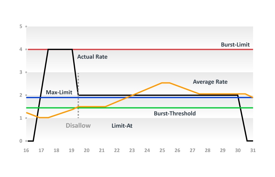
If we decrease burst-time to 8 seconds — we are able to see that in this case, bursts are only at the beginning of downloads The average rate is calculated every 1/16th of burst time, so in this case every 0.5 seconds.
В первой части статьи будет рассмотрен один из механизмов QoS, реализованный в RouterOS, по управлению очередями и пропускной способностью, а именно Simple Queues.
Введение
Одним из способов управления качеством обслуживания в сети является внедрение механизмов QoS (quality of service — качество обслуживания). Использование MikroTik QoS позволяет повысить приоритет трафика одного типа над другим, ограничить полосу пропускания для разных типов трафика. Распространённым сценарием является использование комбинированных методик. В этом случае из общего трафика выделяются потоки в соответствии с заданными критериями и между ними распределяются ресурсы: потокам, для которых важно время обработки, выделяется приоритет в обслуживании, а потокам, для которых важна пропускная способность, выделяется большая гарантированная полоса. Штатные средства RouterOS позволяют выполнить распределение ресурсов между потоками трафика с помощью инструментов Simple Queues (простые очереди) и Queue Tree (дерево очередей).
Следует упомянуть, что конфигурация QoS выполняется на каждом устройстве, поэтому, должна быть распространена на все устройства локальной сети. Эффект от внедрения QoS будет ограничен локальной сетью, поскольку смежные сети, находящиеся под управлением других лиц, работают в соответствии со своими политиками, которые могут не совпадать с вашей.
К важным методам обеспечения качества обслуживания также следует отнести архитектуру построения сети и административные меры. В блок административных мер входит контроль за пользовательским трафиком, в допустимых рамках, и контроль за утилизацией каналов связи и аплинков.

В RouterOS существует несколько типов очередей, управление которыми выполняется в разделе /queue type. Пользователь может создавать свои типы очередей, однако за основу будет браться одна из существующих.
RouterOS поддерживает следующие типы очередей:
1.1 Очередь типа none
Очередь типа none подразумевает под собой использование только аппаратной очереди сетевого интерфейса, через который трафик будет отправлен. Данный тип очереди не позволяет выполнять дополнительные настройки по приоритизации трафика.
1.2 Очереди типа pfifo, bfifo, mq-pfifo
Алгоритм FIFO (first in — first out, первый пришёл — первый ушёл) заключается в том, что данные, попадающие в очередь первыми, будут первыми переданы на дальнейшую обработку. Такой подход не позволяет распределять между потоками данных временные ресурсы в соответствии с их приоритетом и применим, в первую очередь, в системах с невысокой утилизацией каналов передачи данных.
На рисунке 1.1 представлен механизм работы очереди типа FIFO: в очередь поступают пакеты трёх потоков данных. Пакет первого потока поступает в очередь первым и первым из неё выходит, первый пакет второго потока выходит вторым, пакет третьего потока — третьим и второй пакет второго потока — четвёртым.
Рисунок 1.1 — Принцип организации очередей FIFO
Разница между pfifo и bfifo заключается в том, что первый метод применяет алгоритм FIFO попакетно, а второй — побайтово. Очевидно, что данный тип очередей использует единый буфер хранения пакетов, определяемый параметром pfifo-limit и bfifo-limit.
Тип очереди mq-pfifo аналогичен pfifo с той лишь разницей, что использует несколько буферов хранения пакетов для каждого из потоков. Размер буфера определяется параметром mq-pfifo-limit.
В случае переполнения буфера, вновь пришедшие пакеты будут отброшены. Thus, the queue size allows a trade-off between high channel utilization (large queue size) and low latency (small queue size).
1.3 Queue type red
The central concept for RED (random early drop) queues is the average queue size. The user sets the minimum and maximum thresholds red-min-threshold and red-max-threshold and, depending on the position of the average queue size relative to these thresholds, data flow control is performed:
1.4 Queue type sfq
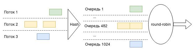
Figure 1.2 — SFQ queuing principle
The queue uses two parameters: sfq-allot is the size of each of the 1024 queues in bytes, sfq-perturb is the time after which the hashing algorithm should be changed.
Thus, it is possible to achieve an equal distribution of bandwidth between all data streams. However, this algorithm has a drawback: if one of the hosts operates with many data streams, it will receive traffic priority over the others, because its traffic will be placed in different queues. In some cases, this can be avoided by choosing the parameters involved in the calculation of the hash function, but this will require changing the queue type to PCQ.
1.5 Queue type pcq
PCQ (per-connection queuing) is an extension of SFQ. As already mentioned, for PCQ, you can select the parameters involved in the calculation of the hash function (the pcq-classifier parameter). In addition, you can set the size of each of the subqueues through the pcq-limit parameter.
One of the advantages of PCQ queues is the ability to flexibly control the available bandwidth for subqueues using the pcq-rate and pcq-total-limit parameters. The pcq-rate parameter sets the throughput threshold for each of the subqueues, and pcq-total-limit sets the total threshold for all subqueues. The bandwidth specified in the pcq-total-limit parameter is evenly distributed among all streams, however, the bandwidth of the stream cannot exceed pcq-rate, even if the channel utilization has a headroom. If there are no thresholds set for the queue, then the available bandwidth will be distributed evenly among the substreams.
A visual demonstration of the effect of the queue size with illustrations is presented in the official documentation — https://wiki.mikrotik.com/wiki/Manual:Queue_Size.
Principles of speed limit
The data flow passing through the interface, whether incoming or outgoing, can be processed in two ways: limiting and equalization (see figure 2.1).
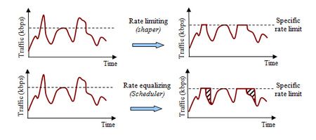
Figure 2.1 — Principle of traffic restriction and equalization
Traffic limit means that all traffic above the specified limit will be dropped. This mechanism is shown in Figure 2.1a — data that exceeds the threshold is discarded. This type of rate limiting is appropriate for traffic that is sensitive to delays: since the data is not stored in a buffer, but is transmitted further or discarded.
Alignment implies a data buffer through which all packets pass within the data stream. If the stream exceeds the specified limits, then the packets are stored in the buffer until it is possible to transfer them further. Such a mechanism is shown in Figure 2.1b — traffic above the threshold is not discarded, but stored in a buffer and transmitted further with a delay. If the stream has reached the specified limit and the buffer is full, incoming packets will be dropped. This approach is used for traffic types that are not sensitive to delays. In addition, such a mechanism equalizes the utilization of communication channels, aligning the data transmission flow.
Based on this, two concepts related to the speed limit are used: CIR and MIR. C IR (committed information rate — guaranteed rate) — the rate that is allocated to the queue in the worst case, but guaranteed. M IR (maximum information rate — maximum speed) — the speed that is allocated to the queue in the best case, if this band is not used by other queues.
In RouterOS syntax, CIR is referred to as limit-at and MIR as max-limit.
2.1 Using Burst
In addition to the rate limiting mechanisms through CIR and MIR, RouterOS has the ability to temporarily increase the bandwidth for the queue, called a burst (impulse, burst).
Operation in burst mode is determined by three parameters, the values of which are set by the user:
The result of using the burst mode is the value of the current data rate (actual-rate) allocated to the data stream.
Consider an example where a user uploads two files, each file is 4 Mb (32 Mb) in size (see Figure 2.2). The loading of the first file starts at zero second, the second — at the seventeenth. The user’s network device is configured as follows:
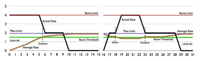
Figure 2.2 — Demonstration of burst mode operation
Time segments are plotted along the abciss axis, and throughput is plotted along the ordinate. Let’s analyze the channel bandwidth allocated to the user in stages:
Thus, the use of burst is useful for improving short-term speed, for example when opening web pages, and increases user loyalty. However, for the burst to work properly, it is necessary to think over its configuration and have a reserve of bandwidth.
Hierarchical token bucket (HTB)
Queuing and their interconnections in RouterOS are performed using the logic of the HTB algorithm (hierarchical token bucket — hierarchical distribution).
The main advantage of HTB is the ability to establish relationships between queues and organize them into a hierarchical structure. Thus, parent-child relationships can be established between queues with inheritance of distributed resources. Within the framework of the HTB algorithm, the concepts of an incoming queue (inner queue) and a final queue (leaf queue) are distinguished. A queue that has at least one child queue is an input queue and is responsible for distributing traffic, while a final queue that has no children is a traffic consumer.
The following parameters can be set for each of the queues: CIR, MIR and priority. The priority will only be used if the CIRs for all destination queues are satisfied and there is some bandwidth remaining. The queue with the highest priority (8 is the lowest priority, 1 is the highest priority) will receive the extra bandwidth first. If the priorities of the final queues are the same, the throughput over CIR will be distributed evenly between them. The allocation of available bandwidth over CIR will be performed only if the priority values are set for the end queues, while the priority of the incoming queue is not taken into account.
When building a hierarchy, one should be guided by the following principles:
The official documentation provides several examples of bandwidth distribution between queues in accordance with the hierarchy (https://wiki.mikrotik.com/wiki/Manual:HTB), let’s analyze one of them (see Figure 3.1).
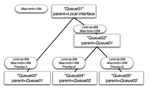
Figure 3.1 — An example of the organization of the queue structure
Bandwidth allocation will be performed according to the following algorithm:
1. Queue03, Queue04, Queue05 reserve 2Mbps according to CIR values;
2. Queue02 reserves 8 Mbps;
3. Since Queue02 has reserved 8 Mbps, of which the end queues Queue04 and Queue05 consume a total of 4 Mbps, the remaining 4 Mbps must be shared between them. To do this, the analysis of the set priority values \u200b\u200bis performed and 4 Mbps is allocated to the Queue04 queue (Queue04 has a higher priority than Queue05);
4. All available bandwidth set as MIR for Queue01 is allocated: Queue03 gets 2 Mbps, Queue04 gets 6 Mbps, Queue05 gets 2 Mbps.
When working with HTB, one should be guided by the following algorithm: at the first stage, the necessary traffic is allocated and marked, then the marked traffic is associated with one of the created queues, and at the last stage, the queue is assigned to a specific interface.
MikroTik Simple Queues
As already mentioned, one of the ways to organize MikroTik QoS in RouterOS is to configure Simple Queues, the configuration of which will be discussed in this section.
MikroTik Simple Queues is a flexible enough tool that allows you to quickly limit the bandwidth for a host, or, using an integrated approach, think through the structure and configure for many networks and data flows.
Setting up simple queues looks like a set of rules and associated policies. The packet processed by the Simple Queues block is sequentially checked for compliance with all rules until the rule is triggered. When triggered, the policies defined by this entry will be applied to the packet. The matching mechanism is similar to the mechanism in Filter, discussed in another series of articles. It follows that a large number of rules leads to an increase in the load on the router’s hardware resources.
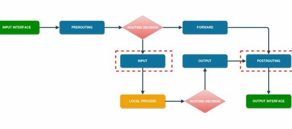
Simple rules can use Mangle’s packet marking. Figure 4.1 shows a simplified packet flow diagram in RouterOS. Packet processing by the Simple Queues block is performed in two stages: Input for incoming packets and Postrouting for outgoing packets (see Figure 4.2). It is important to note that the application of Simple Queues MikroTik is one of the last stages of processing, so marking is performed at any of the stages preceding it. Also, it is important to note that the use of Fasttrack affects the operation of the queues, therefore, as part of the demos, this option will be disabled.
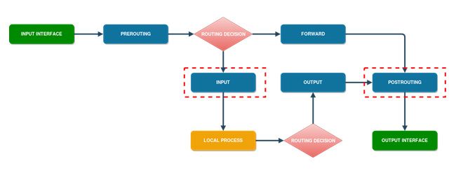

Figure 4.2 — Packet flow diagram for Input and Postrouting chains in RouterOS
4.1 Simple Queues Parameters
Simple rules are configured in the /queue simple section, and when creating rules, you can configure the following parameters:
It is important to understand that if the «target» parameter is not specified, the rate limit will be applied to the traffic twice. This is because in the Packet Flow Diagram (see figure 4.1) the simple rule processing block is present twice and the device will not be able to separate the upload and download streams. Within the framework of the article, the concepts of upload/download are identical to uplink/downlink.
Practice Simple Queues
To demonstrate how to set up simple queues, consider the example in Figure 5.1. Each of the devices in the diagram is a router running on RouterOS. R1 and R2 are traffic consumers — they will run bandwidth-test towards BT_server. Simple queues will be configured on the R_queue router.
Figure 5.1 – Network diagram for case studies
Initial device configuration:
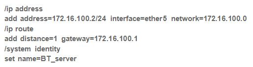
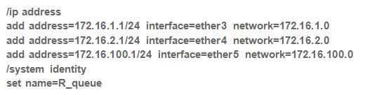
5.1 Subnet rate limit
Let’s set the rate limit for subnet 172.16.1.0/24 upload 10 Mbps, download 5 Mbps. To do this, run the /queue simple add target=172.16.1.0/24 max-limit=10M/5M command on R_queue, and run throughput testing on R1 and R2.
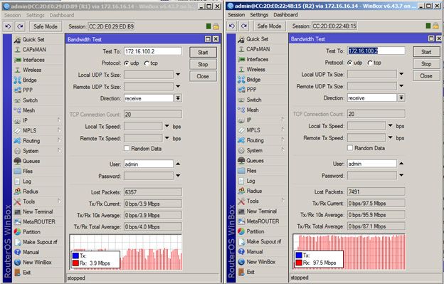
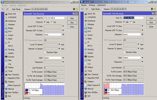
Figure 5.3 — Results of testing in the uplink direction
Figures 5.2 and 5.3 show that consumer R1’s traffic is limited, according to the task, to ~10Mbps/~5Mbps, while R2’s throughput is limited by the port’s physical capabilities.
5.2 Allocation of the total bandwidth by priority
In Example 5.1, the simplest way to limit the rate for a specific subnet was considered. This implementation can be used in small networks, or as a temporary solution. In practice, more often the bandwidth of the channel should be divided among several consumers in different proportions.
To do this, let’s create a hierarchy of simple queues: the parent queue is limited to 10 Mbps, and the child queues are limited to 8 and 5 Mbps, respectively, and have different priorities. It is important to note that the target of the parent queue must match the target of all children.

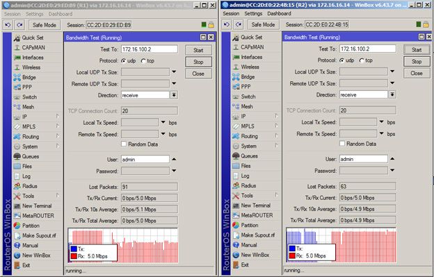
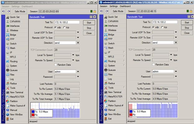
Figure 5.5 — Results of testing in the uplink direction
The bandwidth of the channel is allocated in accordance with priorities — first 5 Mbps is allocated to R2, and then the remaining bandwidth is allocated to R1. R2 does not receive the entire bandwidth of the communication channel, because the limit max-limit=5M is set. At the same time, if you stop consuming traffic on R2, R1 will receive bandwidth in accordance with the restrictions — 8 Mbps:
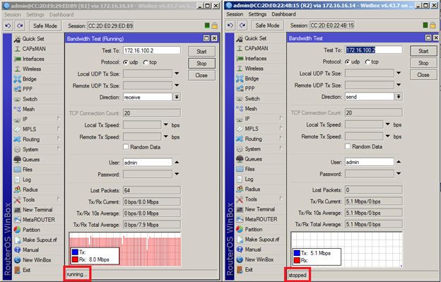
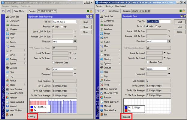
Figure 5.7 — Results of testing in the uplink direction
5.3 Use of CIR and MIR in bandwidth allocation
The disadvantage of the solution considered in example 5.2 is that in the absence of one of the consumers, part of the bandwidth is not used, even if there is a need for it from the side of the active traffic consumer. So, for example, in the absence of R1 traffic, R2 will only be able to use 5 Mbps.
Let’s solve this problem by setting CIR and MIR values. For both consumers, set MIR to 10 Mbps and CIR to 2 Mbps. The priorities will remain the same: the traffic prioritization of the second consumer will be higher.

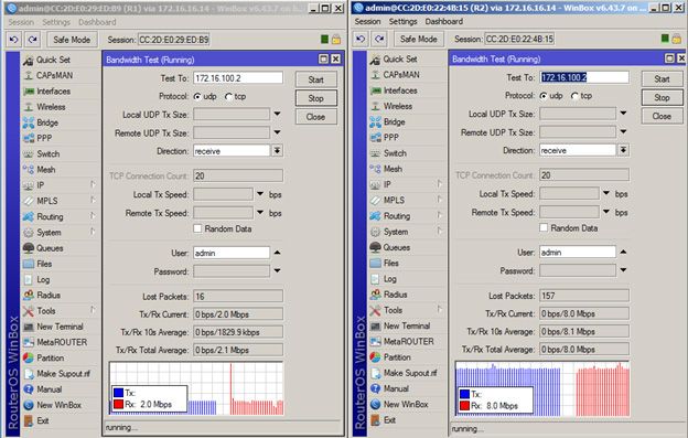
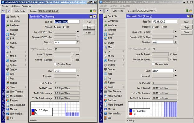
Figure 5.9 — Results of testing in the uplink direction
First, the bandwidth is distributed according to CIR — 2 Mbps, and then, because priority of R2 is higher than that of R1, the rest of the channel bandwidth is given to R2: 10 Mbps — 2 Mbps -2 Mbps = 6 Mbps, i.e. total R2 throughput is 8 Mbps (2 Mbps from CIR + 6 Mbps with channel bandwidth priority). At the same time, if you turn off R2, then R1 starts to utilize the entire available band:
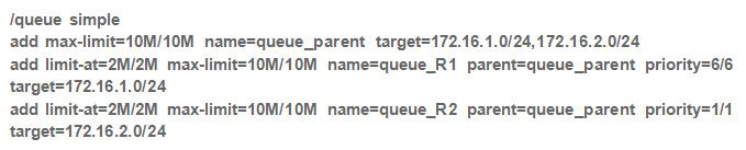
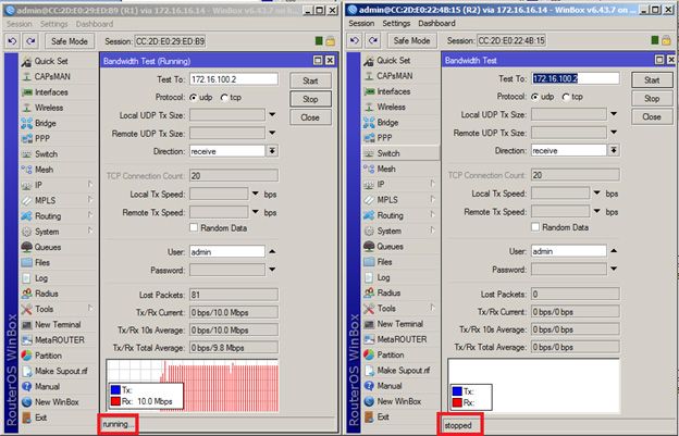
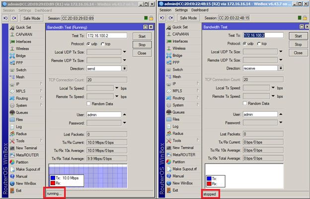
Figure 5.11 — Results of testing in the uplink direction
Conclusion
The first part of the article presents the principles of queuing and their types in RouterOS. The Simple Queues tool is also considered with a demonstration of basic examples of rate limiting. Also, within the framework of practical examples, examples of building a queue structure based on parent-child relationships are considered.
Sharing the Internet or QoS on Mikrotik
The principle of division surrounds us everywhere. This applies to almost every area of our lives. As a rule, we are talking about dividing in equal proportions, which is quite logical.
Modern information technologies, which are responsible for the transfer of large amounts of information, work on the same principle. Dividing algorithms prevent devices from taking more than their allotted amount.
Naturally, we are talking about the Internet. It is he who over the past 15 years has become an integral part of the life of most of the inhabitants of the planet. In the article, we will tell you how to effectively organize the division of the Internet channel (we will indicate the basic settings for system administrators) through the use of the modern RouterOS Mikrotik operating system.
Practice is very important, but without knowledge of the theoretical foundations it will be as difficult as possible to realize what was planned. First, let’s look at a list of key concepts that are simply necessary to solve the issue of shaping — a technology that can effectively limit the speed and quality of Internet access.
Shaper is an algorithm for managing the sequence of presented packets, which will allow you to filter out all those packets that do not fit specifically specified conditions.
Schedulers — an algorithm that controls the movement of the package inside the shaper itself. Forms a priority order of packets, taking into account source addresses and a number of other important parameters. These algorithms include:
Subqueue – a formed queue of packets, which was built according to a pre-selected algorithm.
Queuing discipline (qdisc — queue discipline) — this algorithm allows you to «capture» specific packets, as well as determine the order in which they follow / move.
The basis of shaping in Mikrotik is HTB — a queue discipline, which is implemented in many Linux systems. It is important to study it in order to skillfully manage this algorithm.
In Linux systems, the NTV algorithm was implemented relatively long ago, which determines the discipline of the queue in Mikrotik.
The main features of traffic management in Mikrotik are as follows:
In the HTB discipline, the key concept is the class (rule). A schematic example of a class hierarchy is shown in the image below. In this case, packets with data come from the firewall (Filter), which are distributed to local queues (Self Feed) or sent to queues of parent classes (Inner Feed), depending on the priority, channel load and class parameters. Note that usually at the zero level of the hierarchy there are classes that do not have child rules, they can be called clients. It is these classes that primarily capture traffic, which is then transferred to the parent classes. Two or more classes with the same direct parent have the same level and connection to the same local output queue.
Structure of NTV (schematically)
Each of the classes can have the following parameters:
limit-at — guaranteed speed;
max-limit — speed limit;
priority — class priority.
They also have three different states.
Green, when the upper limit for the throughput of the rule is the limit-at parameter and the movement of packets is carried out according to priorities immediately to the output stream of its level, without moving up the hierarchy.
Yellow, when the rule’s bandwidth exceeds limit-at, but is below the max-limit level. In this case, the rule is disconnected from the output stream of its level and connected to the parent class.
Red, at which the rule’s bandwidth exceeds the max-limit parameter and the rule is disconnected from the parent class with a connection to the local queue.
There are also two types of rules in Mikrotik, which are separated into different tabs in the Winbox utility, which allows you to configure the operating system from under Windows — Simple Queues and Queue Trees.
These rules will be discussed a little later, but now we will give examples of the work of NTV with the creation of several rules.
2 name=Leaf1 parent=ClassA packet-mark=packet_mark1 limit-at=1024000
queue=default priority=8 max-limit=2048000 burst-limit=0
burst-threshold=0 burst-time=0s
3 name=Leaf2 parent=ClassB packet-mark=packet_mark2 limit-at=256000
queue=default priority=7 max-limit=1024000 burst-limit=0
burst-threshold=0 burst-time=0s
1. In the first case, clients 1 and 2 transmit data at a lower speed than the value of the limit-at parameter, and client 3 does not work. In this case, data packets from clients 1 and 2 are queued locally according to their priorities, without passing data to parent classes.
2. In this case, when data is transmitted by the leaf2 client, data is transmitted at a higher rate than limit-at, but at a lower rate than max-limit in its parameters and less than the limit-at parameter for the parent class ClassB . For leaf1, data transfer is carried out at a speed no higher than its own limit-at. In this situation, leaf1 has a higher priority than leaf2, despite specifying a higher priority for the latter in the parameters. The fact is that when transmitting data at a speed exceeding limit-at, client 2 connects to the parent class with priority 8. At the same time, the rule is that the priority of packets at lower levels under the same conditions is higher than at upper ones.

3. In this case, there is an excess of the data transfer rate of client 1 in comparison with the allowable max-limit, and client 2 data is transferred at a speed in the range of more than limit-at and less than max-limit. The third client has a data transfer rate below the limit-at value. In such a situation, it turns out that ClassA is overloaded with data from the first client, which is why ClassB does not have permission to transfer and only the third client remains operational, which connects to the local queue at the zero level.

4. It is also possible that data is simultaneously transmitted by clients leaf1, leaf2, leaf3, ClassB turns yellow, and ClassA turns green. In such a situation, leaf2 becomes the first in the queue at the second level by the right of the highest priority. For clients 1 and 3, this sets a random choice that determines the order.

The flexibility and versatility of the NTV algorithm allows creating on its basis any hierarchies of rules with precise delineation and control of data flows.
Situations are not uncommon when it is required to issue a peak speed to the client for a given time interval. Or it is necessary to send requests and receive data with maximum speed. In such cases, it is necessary to protect other users from problems in the Internet, for which Mikrotik has all the necessary tools.
burst-limit is a parameter that sets the speed available immediately upon connection.
burst-threshold — shows the average speed for the last burst-time seconds;
burst-time — the time required to calculate the burst-threshold.
With these options, and using limit-at with max-limit, you can set the rules for giving the client the maximum speed. For example, let’s set limit-at=128000/128000, max-limit=256000/256000, burst-limit=512000/512000, burst-treshold=192000/192000, burst-time=8 and watch the channel load graph from one client, which is typical for cases with downloading large files via the http protocol.
After the first second, the average channel load is (0+0+0+0+0+0+0+512)/8=64 kbps, which does not exceed the burst-threshold parameter. After the second second, the average speed will be (0+0+0+0+0+0+512+512)/8=128kbps. After the third second, the average speed is already above the burst-threshold, and it drops sharply to max-limit, holding at this level until the average channel download speed reaches a lower value than the burst-threshold parameter.
As soon as this happens, burst speed is issued again.
Scheduler algorithms are usually used in conjunction with shapers, but they can also have rate-limiting features. In fact, the Scheduler is the predecessor of the shaper, providing it with an already prepared queue of packages with the appropriate restrictions set.
Packet/Bytes (FIFO) — based on the principle of primacy (first in, first out) algorithm. It is configured with only one parameter, pfifo-limit (bfifo-limit), which specifies the number of bytes allowed to be stored in the output buffer. If the packets do not get into the buffer, they are destroyed. Below is a graphical diagram of the operation of this algorithm.
SFQ (Stochastic Fairness Queuing) is an algorithm for providing all TCP/UDP connections with the same data transfer capability. This algorithm is applicable for cases with heavy channel load, when it is necessary to provide applications with the same data transmission opportunities. But in practice, it is almost never used, so I will not consider it in detail.
There is also a special case of SFQ in the form of the PCQ (Per Connection Queuing) algorithm, which is responsible for the formation of flows in a subqueue according to specified rules. In theory, such an algorithm could evenly distribute the speed among the participants, regardless of the number of open connections, dividing the bandwidth in equal proportions between classes or clients, which makes it possible to organize dynamic shaping. But an efficient implementation of such an algorithm from the point of view of dynamic shaping has not yet been invented. Nevertheless, thanks to PCQ, it is possible to divide both the incoming and outgoing channels in equal proportions using just a couple of rules.
RED (Random Early Detection) is an algorithm designed to equalize throughput and smooth out jumps with control over the average queue size. When the queue size reaches the red-min-threshold value, a randomly selected package is deleted. The larger the average queue size, the more randomly dropped packets. When the red-max-threshold value is reached, all packages are removed. Such an algorithm is rarely used, and for UDP traffic its use is highly undesirable, since the data may not reach the destination during transmission.
The theoretical introduction is over, now let’s move on to practice.
To begin with, let’s dwell on a special type of Queue Trees, with which you can build a hierarchy of rules and manage packets at the lowest level.
Consider the main controls in Queue Trees:
burst-limit (integer) – parameter responsible for the maximum burst-rate;
burst-threshold (integer) — the parameter responsible for the average channel load, at which it is allowed to issue burst-limit;
burst-time (time) — the element used to calculate the average channel load;
flow (text) — the flow marked in /ip firewall mangle;
limit-at (integer) – guaranteed speed value;
max-limit (integer) – maximum speed indicator;
name (text) – name of the queue;
parent (text) – parent in the HTB class hierarchy;
priority (integer: 1.8) – priority of the queue;
queue (text) – queue type. Specified in /queue type.
I. Let’s create a rule according to which clients of the local or virtual network connect to the conditional site www.test.ru with the maximum speed and minimum response time, while the speed is equally divided between them.
1. First, all packets going from users to the conditional site address 11.222.33.44 and back are marked, which requires the creation of 4 rules. Two of them will label forward and reverse connections, and two more will label packets directly on these connections. It is important to remember that queues are built from packets, and do not work with labeled connections. Therefore, for everything to work, the rules should look like this:
2. Then two types of PCQ queues are created, classified by incoming and outgoing address:
/queue type add name=pcq-download kind=pcq pcq-classifier=dst-address
/queue type add name=pcq-upload kind=pcq pcq-classifier=src-address
3. After that, queues are created that are responsible for incoming and outgoing traffic:
The example shows that only a few rules were enough to implement such a complex task as dynamic shaping for certain addresses that are given peak speed. In most cases, in practice, everything is more complicated with a large number of combined rules.
In Queue Trees, in fact, all actions are built on the speed limit, and source addresses, ports, protocols and other parameters are entered in the Mangle firewall section. This method allows you to provide good ping to certain addresses even in cases where there is a serious load on the channel.
Let’s give an example of such rules for the conditional server www.ptimer.ru.
Four rules need to be written in the Firewall, in the first of which all connections with the recipient address 111.333.22.44 are marked with the name primer-connection-up. The second rule labels packets in primer-connection-ups with the name primer-packet.up. We also mark all connections with source address 111.333.22.44 with the name primer-connection-from and the packets in these connections with the name primer-packet-from.
/ip firewall mangle add chain=prerouting dst-address=111.333.22.44 action=mark-connection new-connection-mark= primer-connection-up passthrough=yes/ip firewall mangle add chain=forward connection-mark= primer-connection-up action=mark-packet new-packet-mark= primer-packet-up passthrough=yes
/ip firewall mangle add chain=prerouting src-address=111.333.22.44 action=mark-connection new-connection-mark= primer-connection-from passthrough=yes
/ip firewall mangle add chain=forward connection-mark= primer-connection-from action=mark-packet new-packet-mark= primer-packet-from passthrough=yes
Then two rules are created in Queue Trees for incoming and outgoing flows
/queue tree add name=queue1 parent=global-out packet-mark= primer-packet limit-at=0
queue=default priority=1 max-limit=50000 burst-limit=0 burst-threshold=0
burst-time=0s /queue tree add name=queue2 parent=global-in packet-mark= primer-packet-from limit-at=0 queue=default priority=1 max-limit=50000 burst-limit=0 burst-threshold =0
burst-time=0s
Thanks to these rules, packets arriving and departing from the address 111.333.22.44 are sent to priority queues and always have a guaranteed speed of 50 Kbit/s. Using such a scheme, for example, you can set a fixed guaranteed speed for online games by distributing the bandwidth equally among all network participants.
Simple Queues are simplified because they do not require the use of tagged packets from the Firewall. But the high flexibility in the settings is lost. The main parameters for creating rules here are the source and destination addresses.
We can single out a list of the main features of simple queues.
· Ability to work with P2P traffic.
· Using queues for specific time slots.
· Ability to prioritize streams.
· Use as options multiple chains of packets marked in the /ip firewall mangle.
Create one rule for outgoing and incoming flow.
You can also specify the Parent parameter in Simple Queues, which allows you to build a class hierarchy almost the same as in Queue Trees. The difference is that addresses are used here, not packets and streams. At the same time, Simple Queues have always been and remain a special case of Queue Trees. This means that when creating new rules in simple queues, you should check for similar rules with the same ports, addresses, or other parameters in Queue Trees. If the rules are similar, priority remains with Queue Trees and simple queues do not work.
When you start creating rules in Simple Queues, remember that there is outgoing and incoming traffic for clients, router and provider. Let us show schematically in the figure the direction of traffic flows from the provider to the router, from the router to the client and in the opposite direction. It turns out that outgoing client traffic is incoming for the router and vice versa.

Note that having the ability to manage incoming and outgoing traffic allows clients to use the channel as efficiently as possible.
Imagine a channel for a client with a speed of 128/64 kbit/s, with a guaranteed speed of 64/32 kbit/s on weekdays. As well as a channel with a speed of 512/256 kbit/s with a guaranteed speed of 128/128 kbit/s on weekends.
The result of our work will be two rules:
/queue simple add target-addresses=192.168.11.1/32 limit-at=64000/32000 max-limit=128000/64000 time=00:00:00-00:00:00,mon,tue,wed ,thu,fri/queue simple add target-addresses=192.168.11.1/32 limit-at=128000/128000 max-limit=512000/256000 time=00:00:00-00:00:00,sat,sun
In the 32000/32000 pair, the first digit is responsible for the incoming channel for the client, and the second for the outgoing channel. If you want to ensure fast opening of pages, add burst-limit and burst-time.
It is also possible to modify this rule in order to share the specified speed between the entire network 192.168.11.0.24. In this situation, the queue parameter needs to be set to the pcq-download queue type, which was shown in the Queue Trees example above.
Thanks to simple queues, it is easy to implement the provision of unlimited speed to certain addresses. For example, according to the following rule, a client with the address 192.168.11.1 gets access to the address 88.205.221.123
at a speed of 1 to 2 megabits
/queue simple add target-addresses=192.168.11.1/32 dst-address=88.205.221.123 limit-at=1024000/1024000 max-limit=2048000/2048000
If a guaranteed bandwidth is allocated for an individual client, remember that the sum of the limit-at of all clients cannot exceed the bandwidth of the entire channel.
It can be noted that Mikrotik has a built-in ability to synchronize time with an external source, which is relevant for cases with incorrectly set clocks or a dead battery on the motherboard.

Mikrotik has great traffic management capabilities, which allows this system to stand on a par with popular hardware solutions from Cisco, and in some ways even surpass them. Thanks to the combination of Mikrotik and billing with support for the Radius protocol, a powerful system is obtained that can work both as a distributing Internet server within the local network and in the network of an average provider. Thanks to the shaping capabilities described in the article, you can not only share Internet access, but also create backup communication channels. Adding RouterOS wireless technology turns a few wireless NICs and some hardware into a powerful Wi-Fi system that provides guaranteed bandwidth to split clients.
Applies to RouterOS: v2.9 and newer
Burst is a feature that allows to satisfy queue requirement for additional bandwidth even if required rate is bigger that MIR (max-limit) for a limited period of time.
Burst can occur only if average-rate of the queue for the last burst-time seconds is smaller that burst-threshold.
Burst will stop if average-rate of the queue for the last burst-time seconds is bigger or equal to burst-threshold
Burst mechanism is simple — if burst is allowed max-limit value is replaced by burst-limit value. When burst is disallowed max-limit value remains unchanged.
Values: limit-at=1M , max-limit=2M , burst-threshold=1500k , burst-limit=4M
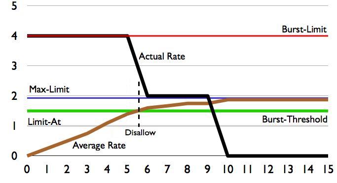
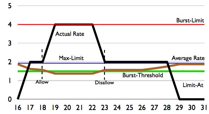
Average rate is calculated every 1/16 of burst time, so in this case 1s
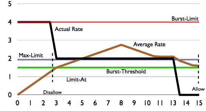
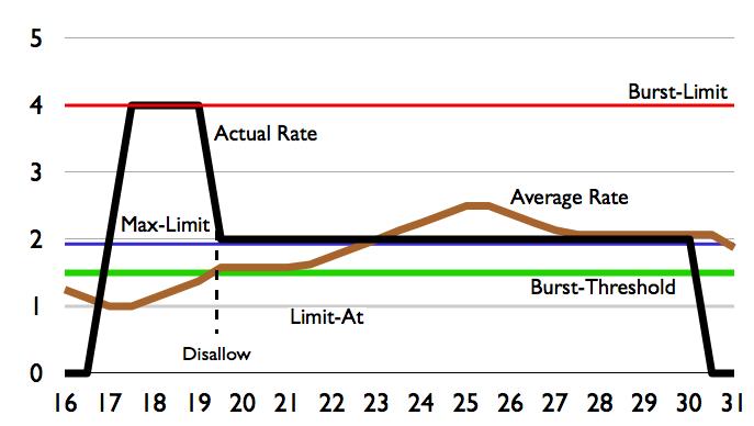
If we decrease burst-time to 8 seconds — we are able to see that in this case bursts are only at the beginning of downloads